This article was published in Scientific American’s former blog network and reflects the views of the author, not necessarily those of Scientific American
In “The Chemical Basis of Morphogenesis,” Alan Turing proposed that chemical substances (morphogens) can transform and spread through tissue to yield natural patterns—stripes, spots and spirals—seen on animals. Turing expressed this idea in the language of differential equations, whose initial conditions controlled the evolution of the patterns.
The complexity and detail in the patterns from such reaction-diffusion systems can be truly surprising—a relatively simple process and small number of parameters can yield an endless variety of familiar patterns and shapes. One season-appropriate example of this is snowflakes, known for their variety and complexity.
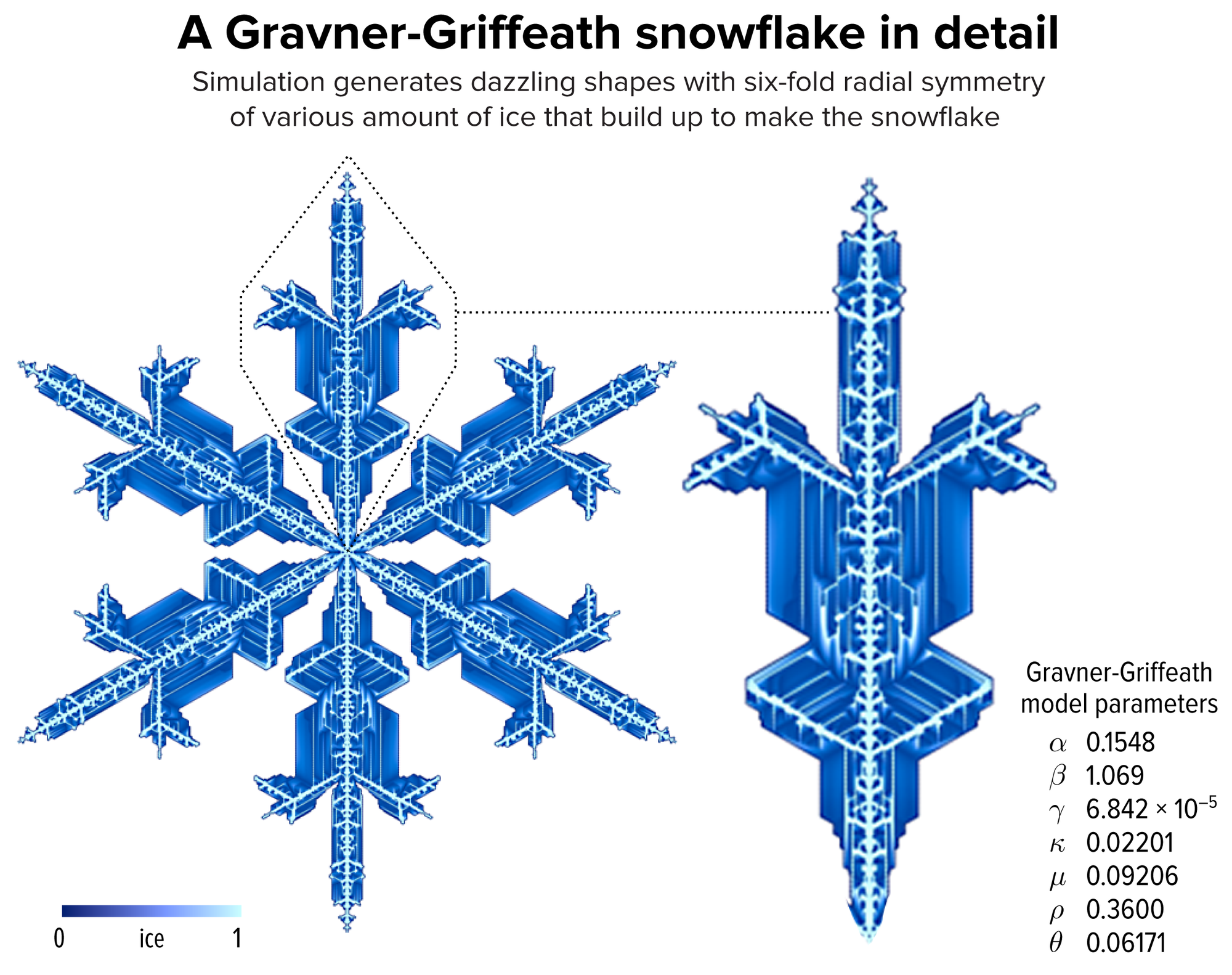
Figure 1. An example of a snowflake grown using the Gravner-Griffeath model. Various amounts of ice (encoded by the blue tone) at different parts of the snowflake make up the six-fold radially symmetric shape. You can browse the details about this snowflake in our online snowflake collection. Credit: Martin Krzywinski and Jake Lever
On supporting science journalism
If you're enjoying this article, consider supporting our award-winning journalism by subscribing. By purchasing a subscription you are helping to ensure the future of impactful stories about the discoveries and ideas shaping our world today.
Compellingly realistic snowflakes can be simulated using the Gravner-Griffeath model, which you can run yourself with code made available by the authors (Figure 2). The snowflake’s radial symmetry is inherited from the hexagon grid on which it grows. Three different kinds of mass are simulated at different grid sites: ice, quasi-liquid and vapor. Initially, ρ amount of ice is initialized at a snowflake site and ρ vapor mass everywhere else. The model then transports and transforms a fraction of these masses by diffusion, freezing (controlled by κ) and melting (controlled by μ and γ). For example, during freezing a fraction κ of vapor at a boundary mass becomes ice and the remaining fraction 1–κ becomes quasi-liquid. Boundary sites around the snowflake become part of the snowflake through a process of attachment, which is controlled by the parameters α, β and θ, which act as cutoff values. Once a site becomes part of the snowflake, all of its mass becomes ice that no longer changes.
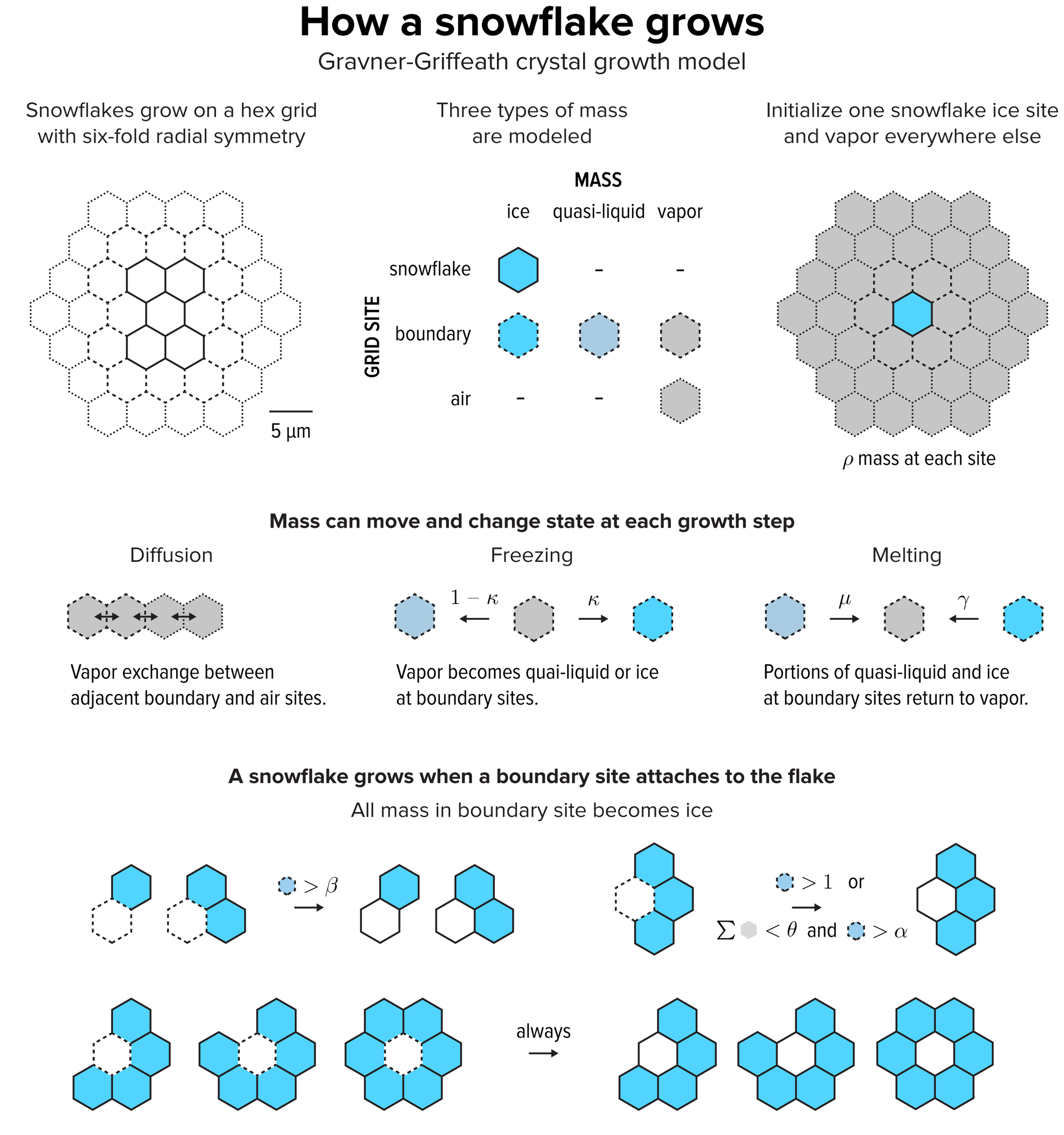
Figure 2. The Gravner-Griffeath model is a type of reaction-diffusion system, with three kinds of “morphogens”: ice, quasi-liquid and vapor. The model is deterministic—given a set of parameters the output is always the same. Optionally the model can include randomness by perturbing the amount of vapor mass in every site at each step. Credit: Martin Krzywinski and Jake Lever
All our snowflakes were grown on an 800 × 800 hexagonal grid for up to 30,000 growth steps and are presented here on a rectangular grid, obtained by rotating and scaling. Snowflakes are always initialized with a single site at the center the grid and were considered to have grown to full size when they reached close to the boundary of the grid, at which point the simulation ends. In Figure 3 we follow the growth of the snowflake from Figure 1. The color map was chosen to highlight the boundary of the flake when drawn on a light background—note that light blue represents high mass while dark blue represents low mass.
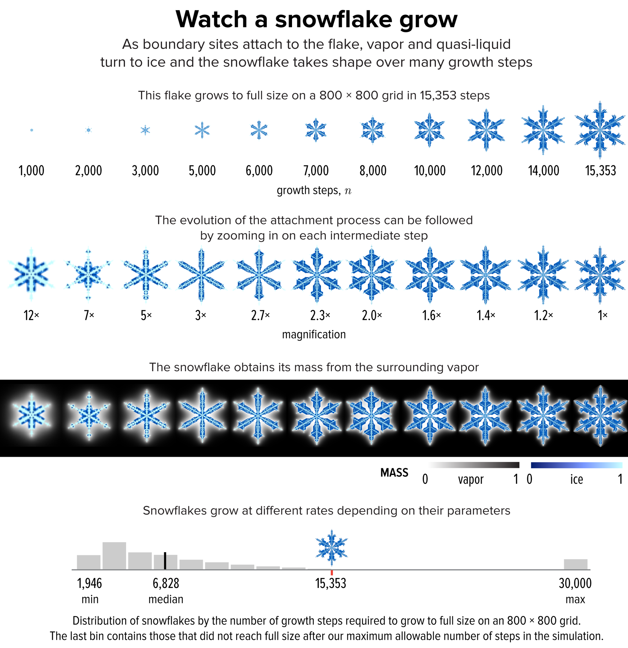
Figure 3. The evolution of the snowflake from Figure 1 to full size at 15,353 growth steps. Credit: Martin Krzywinski and Jake Lever
The snowflake in Figure 1 took 15,353 steps to grow to full size. The rate of growth can be seen in the first row of images in Figure 3. In the second row, each image is magnified by different amount to better reveal the details of the growth in the smaller snowflakes. Remember that once a site joins a flake its mass is fixed for the duration of the simulation. Initially, the ice mass accumulates along the axes of symmetry and quickly tiny bumps begin to appear. These grow into branches because vapor doesn’t have to diffuse as far to reach the bump as the rest of the snowflake. This process is called branching instability and gives rise to dendritic snowflakes.
The snowflake grows quickly at the inside corners because the attachment process is automatic for boundary sites that have more than 3 snowflake neighbors. This gives deposits a small amount of mass (dark blue) to fill in the snowflake. This is called faceting and it is the opposite of branching. Faceted snowflakes have simple flat surfaces. By 2,000 iterations we see that branching slows down and more and more facets appear (dark blue).
The role of the vapor can be seen in the third row of images, which depicts the amount of vapor mass in each air site using a grey scale. The amount of vapor impacts the formation of ice through freezing (κ), melting (γ) as well as attachment, where a boundary cell with three snowflake neighbors can attach if the amount of vapor in its neighborhood is less than θ and the amount of quasi-liquid is higher than α.
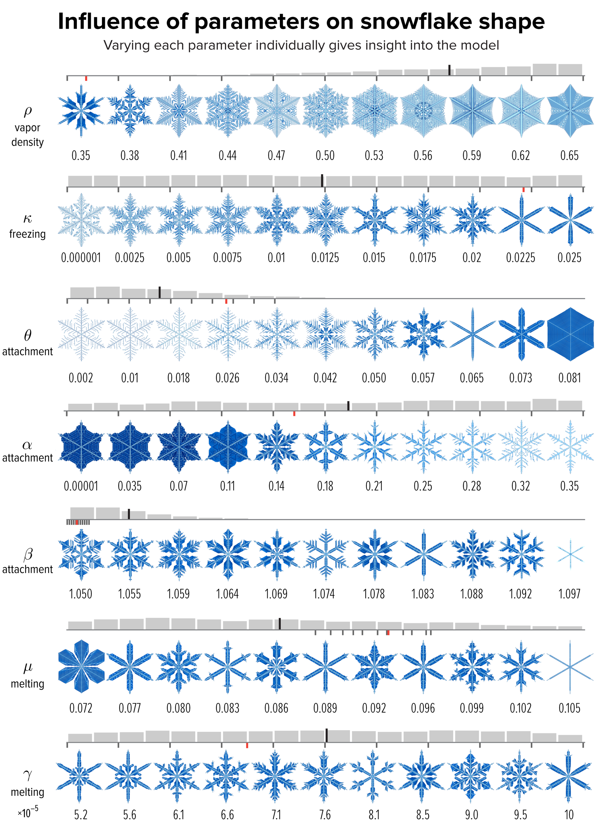
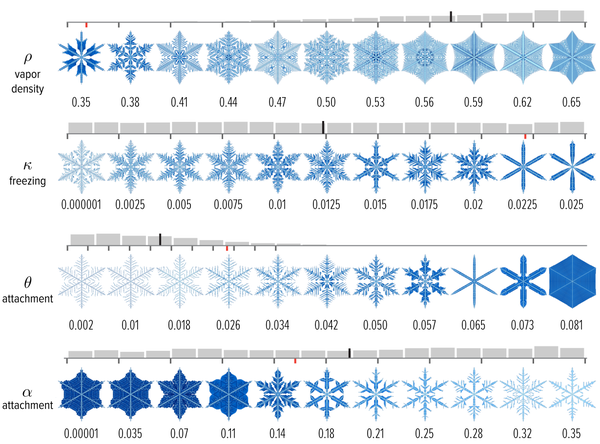
Figure 4. The effect of varying each of the model parameters on the shape of the snowflake in Figure 1, whose parameter value is shown as a red dot. The images sample the parameter values shown by small black ticks. The distribution of snowflakes in our collection by parameter value is shown as a gray histogram. The median is the long black line among the bins. Credit: Martin Krzywinski and Jake Lever
Despite the fact that the model is relatively simple, the effect of the parameters on the shape of the snowflake is quite complicated. To see how the parameters impact shape, we used the snowflake in Figure 1 as a control and varied each of its parameters systematically across the range of viable snowflakes. By “viable” we mean snowflakes that didn’t grow into trivial hexagons and occupied more than 60% of the hex grid after 30,000 iterations—these kinds of snowflakes represent about 10% of those grown with randomly generated parameter values.
For example, increasing ρ, which controls the total amount of mass, increases the speed of growth and encourages branching. Our snowflake in Figure 1 had a low value of ρ and hence not as many branches. Increasing θ and decreasing α both encourage faceting, because these parameters are cutoffs for attachment.
Given the large amount of variation in shapes in Figure 4, it’s reasonable to try to cluster snowflakes based on similarity. Complex systems of snowflake classification have already been proposed. These include categories like sectored plates (simple hexagons, θ = 0.081 in Figure 4), stellar plates (full star-like snowflakes, μ = 0.072 in Figure 4), stellar dendrites (branched snowflakes, α = 0.18 in Figure 4) and fernlike stellar dendrites (highly branched, ρ = 0.5 in Figure 4). It’s interesting to see each of these classes can be obtained in several ways by varying a single parameter from the flake in Figure 1, which is a stellar dendrite.
There are two options of grouping the snowflakes: by parameter value or by shape. Originally, our plan was to create grouping by parameter, which we felt was closer to the internal workings of the model. However, as Figure 4 shows, the parameter space is quite chaotic—small changes in parameters can create large differences in shape. We chose therefore to use shape, which we hoped would create more visually pleasing groups, which we could later relate to parameter values (Figure 5).
Since we grew our snowflakes on an 800 × 800 grid, each snowflake can be considered as vector of length 640,000, in which values are the vapor or ice mass. Snowflakes with similar vectors (as measured by Euclidian distance) have similar shape. But, with our collection of about 15,000 snowflakes, clustering such large vectors was computationally infeasible. We addressed this by down-sampling the snowflakes by a factor of five to create a 160 × 160 grid, which we further blurred with a Gaussian filter to smooth out small differences between similar snowflakes. The similarity between any pair of snowflakes was the Euclidian distance between the corresponding 25,600-element vector.
Using this similarity between snowflakes is calculated, we have a sense of their “distance.” Unfortunately, this distance is expressed in a space with 25,600 dimensions. To visualize this space, it is customary to dimensionally reduce this space to two dimensions, allowing us to draw it on the page.
A common approach to this is principal component analysis (PCA), which identifies the axes of greatest variance within a dataset and rotates the data so that the first dimension shows the greatest variance. Essentially, the rotation is picked so that trends in the data are preserved as much as possible. PCA assumes a linearity to the data set, which is certainly violated by our snowflakes. Nevertheless, PCA identifies θ (attachment) and ρ (mass) as highly correlated with the first two principal components. This does separate the snowflakes by their “fullness” but isn't able to tease out smaller groupings.
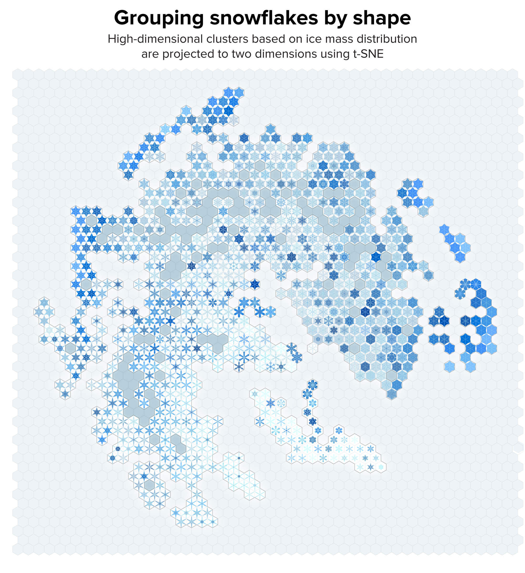
Figure 5. Our collection of snowflakes clustered based on structural similarity. Clusters are projected onto two dimensions using t-SNE. The snowflakes are themselves arranged on a hex grid to allow tighter packing. Credit: Martin Krzywinski and Jake Lever
An alternative to PCA is t-distributed stochastic neighbor embedding (t-SNE). This method uses the principle that similar snowflakes in the high-dimensional space should be placed close together in the low-dimensional space. It models the similarity of two snowflakes as a probability distribution in both high-dimensional space and low-dimensional space and minimizes the difference between these two distributions. Let dij be the Euclidian distance between snowflakes i and j, then

is the conditional probability of picking snowflake j as a neighbor of snowflake i.
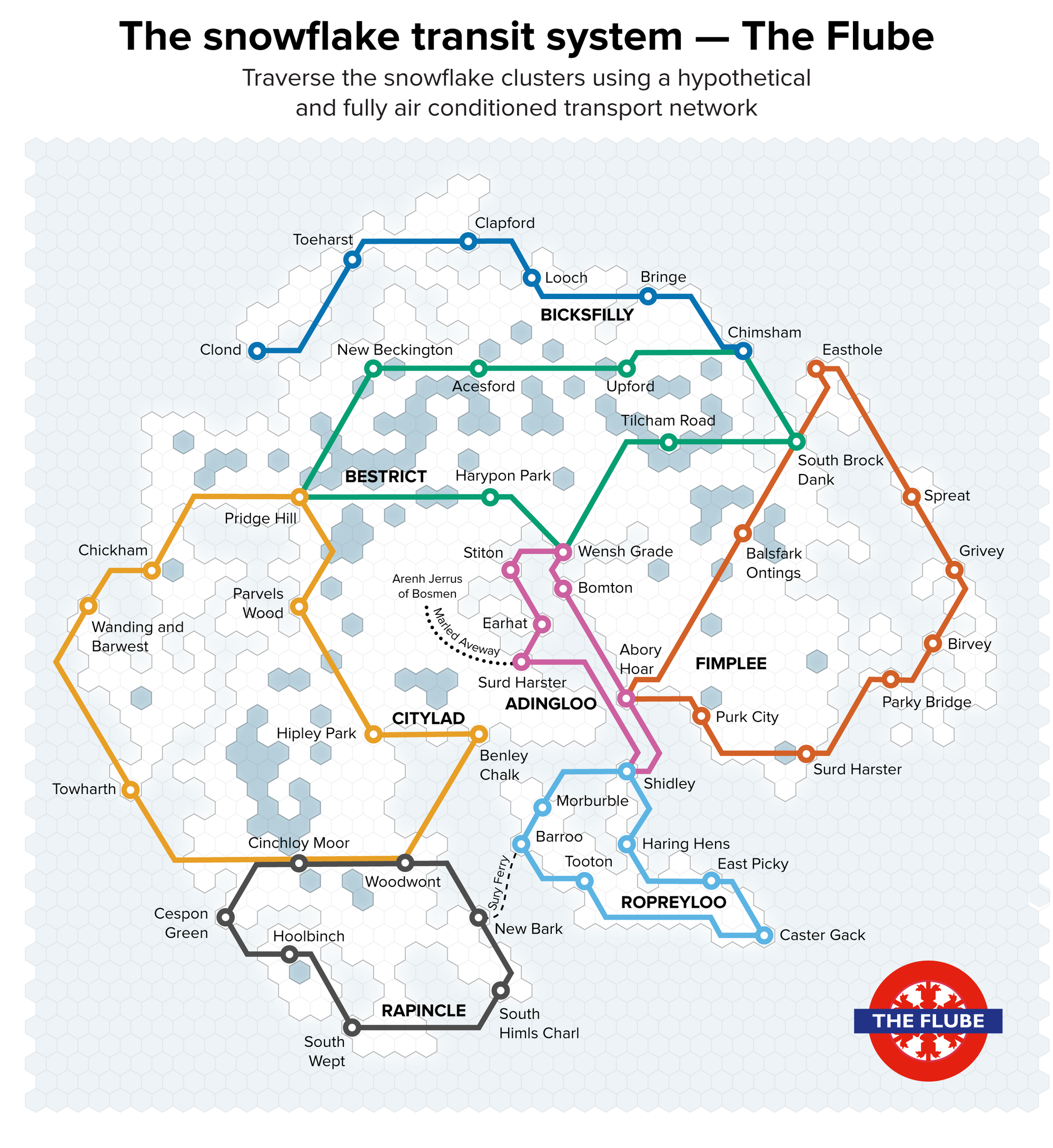
Figure 6. A collection of paths in the two-dimensional t-SNE space of the snowflakes, affectionately named “The Flube.” Credit: Martin Krzywinski and Jake Lever
Having already built a snowflake world with t-SNE—a mapifying process generally helpful in concretely illustrating relationships between clusters—we thought to expand this imaginary land to have its own transit system, which would form a network across this continent to allow snowflakes to transit across areas. Naturally, we named this system “The Flube” (Figure 6).
Since the snowflakes are simulated, we also simulated names for the lines and stations in The Flube using a recurrent neural network (RNN) trained on the names of 622 London Underground and rail stations. We grouped the names into lines based on their perceived personality: Ropreyloo is playful with stations like East Picky and Morburble, Citylad is posh with Benley Chalk and Wanding & Barwest and stations like Bringe and Clapford along Bicksfilly are not likely to be popular tourist destinations.
The RNN is a more sophisticated version of a Markov model, which is a finite state automaton that can generate a letter (or a word) based on specific probabilities learned from a training set of letters (or words). The probability of transition is only based on the current state of the machine and doesn't use all the previous output. An RNN, on the other hand, combines a traditional neural network with an internal state. This state keeps track of all the previous inputs to the network and hence remembers the previous letters in the generated word. The RNN concept has been used to generate Shakespeare-like English, recipes and rap lyrics.
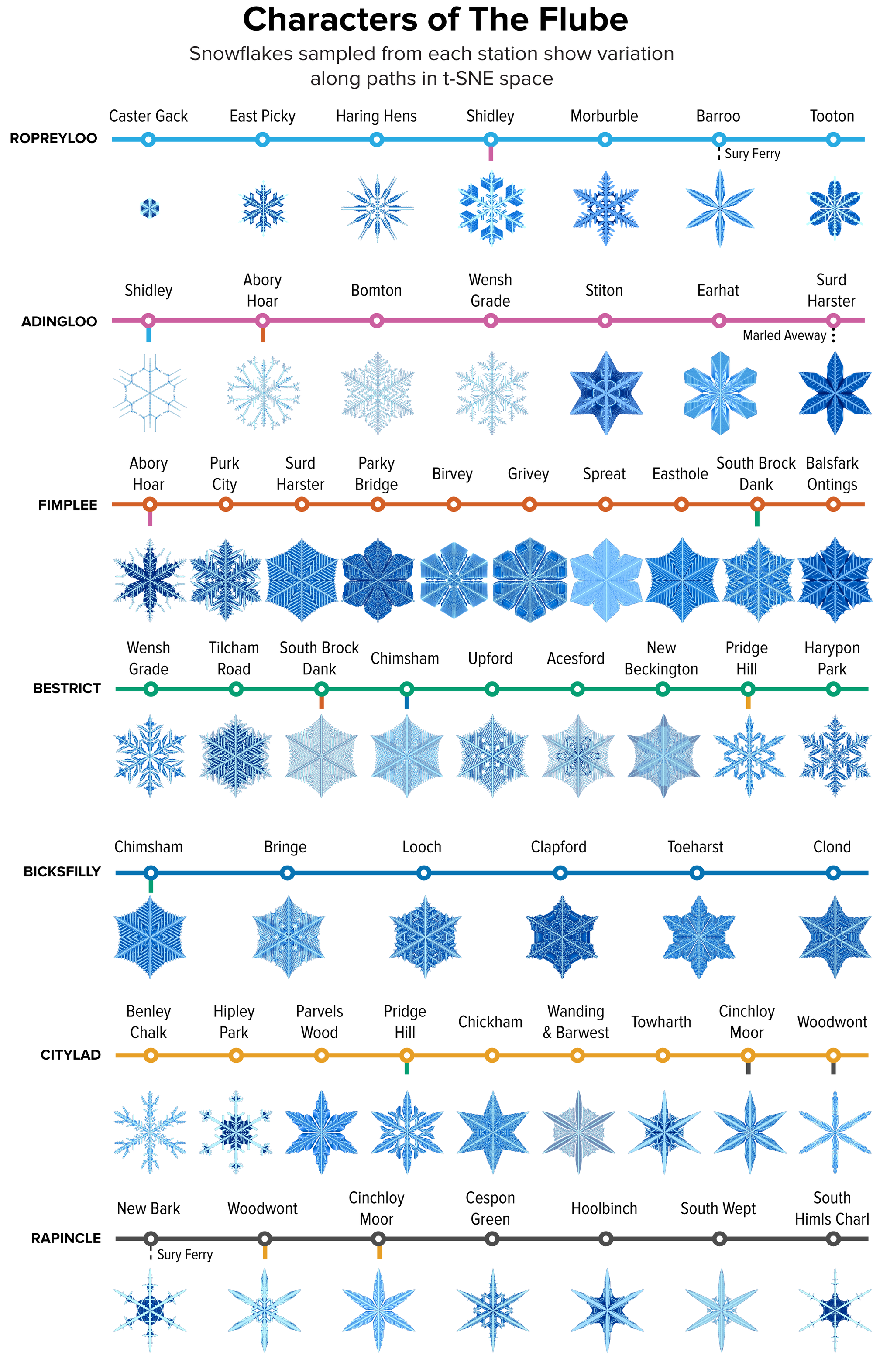
Figure 7. A sample of the snowflakes found at the t-SNE hex grid of each station in The Flube, showing the variation in shape within and between clusters. Credit: Martin Krzywinski and Jake Lever
We can use the Flube lines and stations to sample the t-SNE space (Figure 7), much like the sampling of parameter space shown in Figure 2. We assigned the line and station names in keeping with our impression of the shape of the snowflakes. The smaller (young) snowflakes were assigned the playful Ropreyloo line while the snowflakes in the north, which we thought of as a remote and harsh land, got Bicksfilly. It’s a long trip from Caster Gack to Clond (four transfers are required: Shindley, Abory Hoar, South Brock Dank and Chimsham).
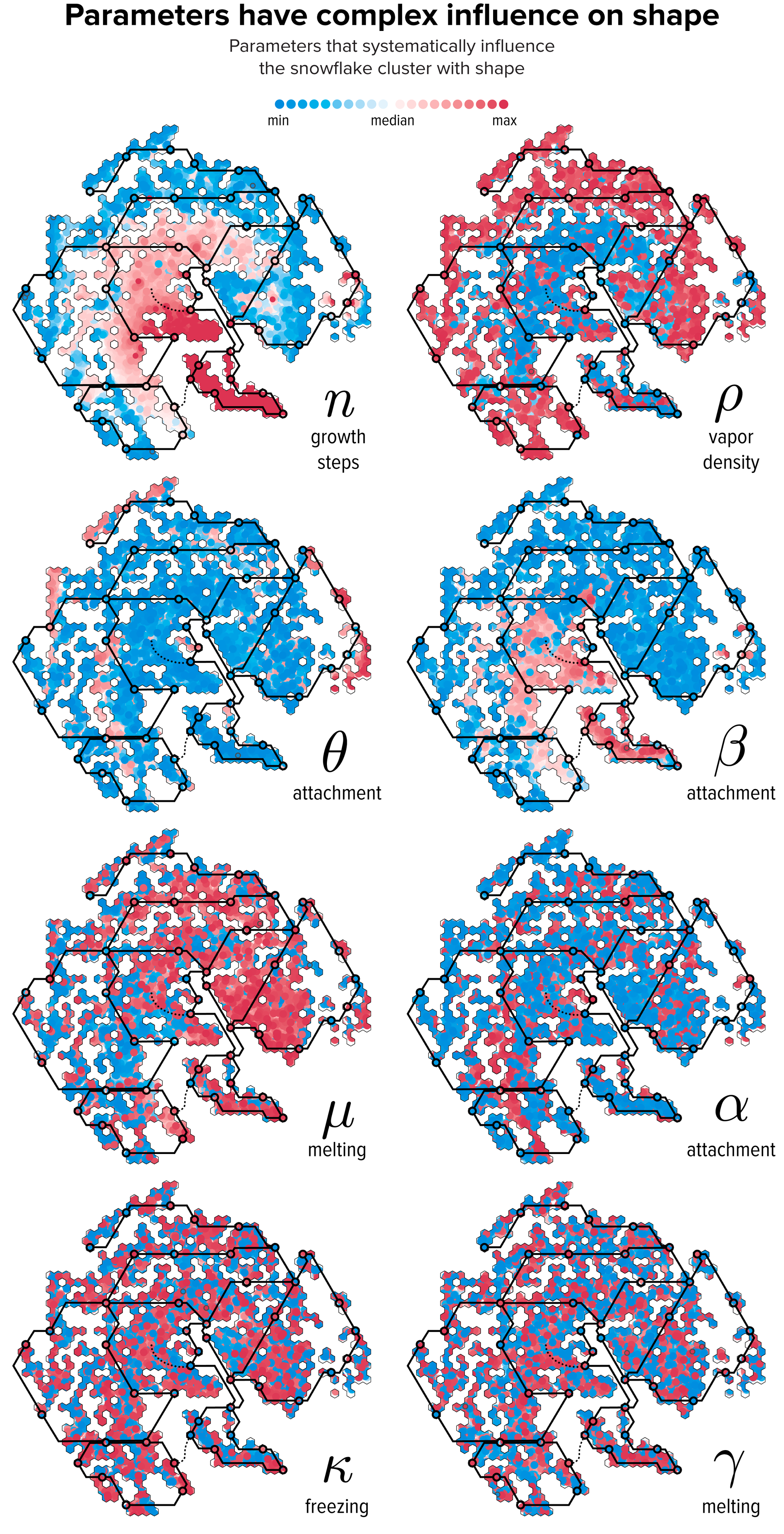
Figure 8. The relationship between parameter values and t-SNE clustering. Each snowflake is drawn as a circle colored by the relative difference of the snowflake’s parameter with the median value. The lines of The Flube are superimposed to help interpret the variation in shape in Figure 7. Credit: Martin Krzywinski and Jake Lever
Figure 8 makes the connection between parameter values and the t-SNE clustering. The snowflake shapes on the t-SNE continent can now be interpreted by their parameters. For example, the island to the south (Ropreyloo) with small snowflakes corresponds to low θ and low ρ, high α and high β. The peninsula to the north (Bicksfilly) and island groupings to the east (Fimplee) with stellar plate snowflakes (high θ). The center of the land mass (Bestrict) was composed largely of fernlike dendrites (low ρ) and the southwest subcontinent (Rapincle) had many stellar dendrites (low α).
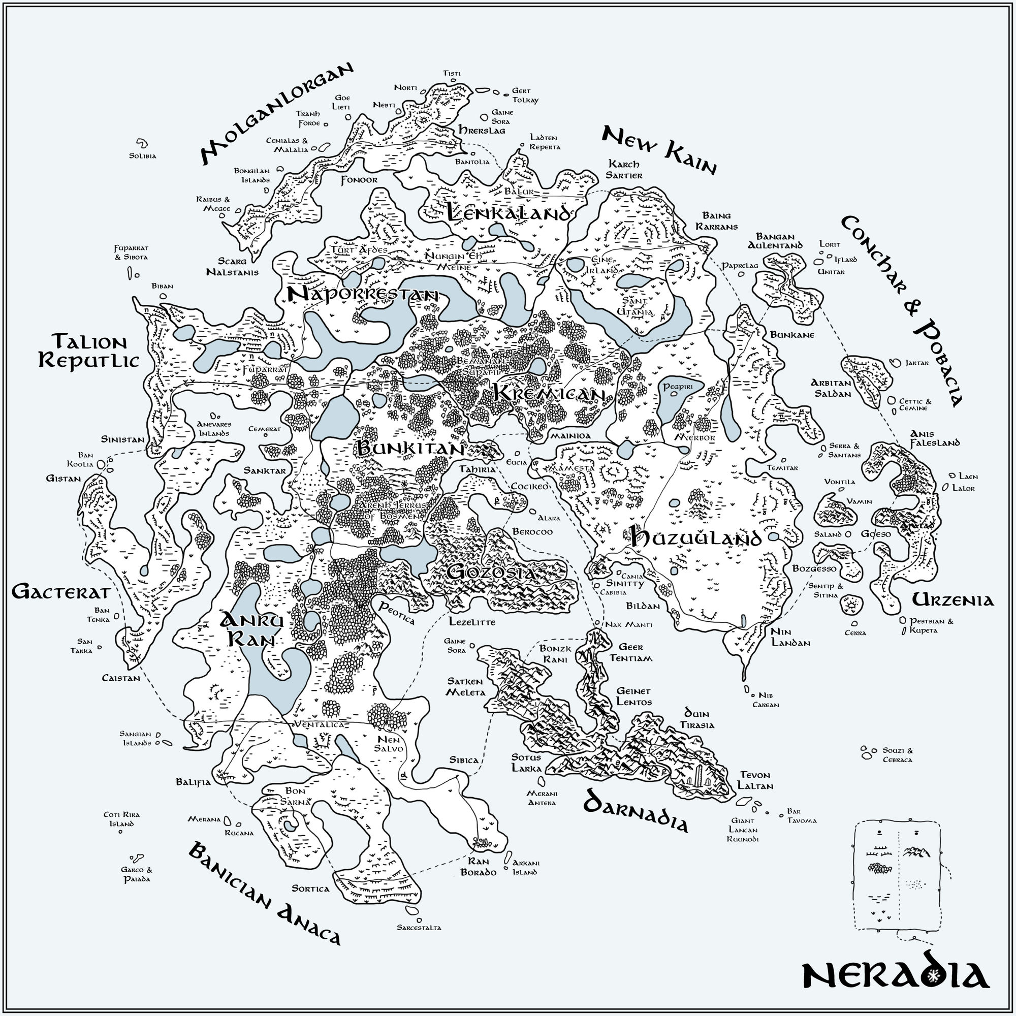
Figure 9. A hand-drawn interpretation of the t-SNE map in Figure 5. Geographical features encode parameter values: woods (low ρ), grassland (low β), marsh (low μ) and desert (high θ). The speed at which the snowflake grew (steps to reach full size, n) is encoded by mountains (high n) and ice cliffs (low n). All names are generated using an RNN trained on 257 names of countries. The Flube network is drawn as thin lines with stations as loops with cities (medium size text) placed at the location of station positions in Figure 6. Credit: Martin Krzywinski and Jake Lever
Once we had created the transit system, the next step was to imagine a whole world, which we called Neradia. By encoding parameter values as geographical features and using an RNN trained on 257 country names we generated a hand-drawn version (Figure 9) of the t-SNE map in the style of Tolkien.
Even with a small training set like the 257 country names, the RNN output was extremely entertaining. Our favorites are regions of Conchar & Pobacia (northeast) and New Kain (north). The location of each station in The Flube was assigned a city name in keeping with the flavor of the station name. Clapford station is in the city of Hrerslag in the region of Molganlorgan and Abory Hoar is in the city of Sinnity in the region of Huzuuland. Curious RNN slips of the letter such as “islands” to “inlands” appear in the “Anevares Inlands”, which are a set of islands deep within the region of Talion Reputlic (a hilarious misspelling).
We’ve explored generating other text with RNNs in a collection we call the “unwords.” Your friends discouraged you from naming your first daughter Ginavietta Xilly Anganelel but you didn't listen. When you named your second daughter Nabule Yama Janda everyone wanted to know what your secret to having such successful children was. There’s plenty of choice for boys too: Babton Laarco Tabrit and Ferandulde Hommanloco Kictortick. Let’s hope none suffer from myconomascophobia, are never bitten by a cakmiran and aspire to be gabdologists.
The sample snowflake in Figure 1 was assigned the RNN output of Arenh Jerrus of Bosmen and drawn on the map based on its t-SNE position in the woods of the region of Bunkitan. The flake is important enough on The Flube map to have its dedicated connection called the Marled Aweway, which originates at Surd Harster on the Adingloo line.
Next time you’re in a snowstorm or hard at work shoveling (snow), say hello to the denizens of Neradia and think of a story to tell about your own data.
We’d like to thank Lisa Shiozaki and Rodrigo Goya for helpful discussions. High-resolution versions of the images included in this post can be viewed on Krzywinski's website.