A Deep Dive into Deep Learning

This article was published in Scientific American’s former blog network and reflects the views of the author, not necessarily those of Scientific American

On Wednesday, March 27, the 2018 Turing Award in computing was given to Yoshua Bengio, Geoffrey Hinton and Yann LeCun for their work on deep learning. Deep learning by complex neural networks lies behind the applications that are finally bringing artificial intelligence out of the realm of science fiction into reality. Voice recognition allows you to talk to your robot devices. Image recognition is the key to self-driving cars. But what, exactly, is deep learning?

Dozens of articles tell you that it’s a complex, multilayered neural network. But they don’t really shed much light on deep learning’s seemingly magical powers. For example, to explain how it can recognize faces out of a matrix of pixel values (i.e., an image).

As a data science educator, for years I have been seeking a clear and intuitive explanation of this transformative core of deep learning—the ability of the neural net to “discover” what machine learning specialists call “higher level features.” Older statistical modeling and machine learning algorithms, including neural nets, worked with databases where those features with predictive power already exist. In predicting possible bank failure, for example, we would guess that certain financial ratios (return on assets, return on equity, etc.) might have predictive value. In predicting insurance fraud, we might guess that policy age would be predictive.

On supporting science journalism

If you're enjoying this article, consider supporting our award-winning journalism by subscribing. By purchasing a subscription you are helping to ensure the future of impactful stories about the discoveries and ideas shaping our world today.

With tasks like voice and image recognition, structured informative predictor information like this is not available. All we have are individual “low-level” sound wave frequency and amplitude, or pixel values indicating intensity and color. You’d like to be able to tell the computer “just look for two eyes,” and then provide further detail on how an eye appears—a small solid circle (pupil), surrounded by a ring (iris), surrounded by a white area. But, again, all the computer has are columns of (low-level) pixel values; you’d need to do a lot of extra work to define all the different (higher-level) pixel patterns that correspond to eyes. That’s where deep learning comes in—it can “learn” how to identify these higher-level features by itself.

As I looked for explanations of how this works, I found that most narratives dissolve vaguely at the key point, often with an image of circles in columns, and lots of lines connecting the circles. It’s as if the lecturer, who has held you spellbound to this point, waves his hands in the air and says “and that’s how higher-level features like faces are discovered.”

Then I attended a workshop and learned about convolutions.

CONVOLUTIONAL NEURAL NETWORKS (CNNs)

In a standard neural network, each predictor gets its own weight at each layer of the network. A convolution, by contrast, selects a subset of predictors (pixels), and applies the same operation to the entire subset. It is this grouping that fosters the automated discovery of features. Recall that the data in image recognition tasks consist of a large number of pixel values, which, in a black and white image, range from zero (black) to 255 (white). Since we are interested in detecting the black lines and shadings, we will reverse this to 255 for black and zero for white.

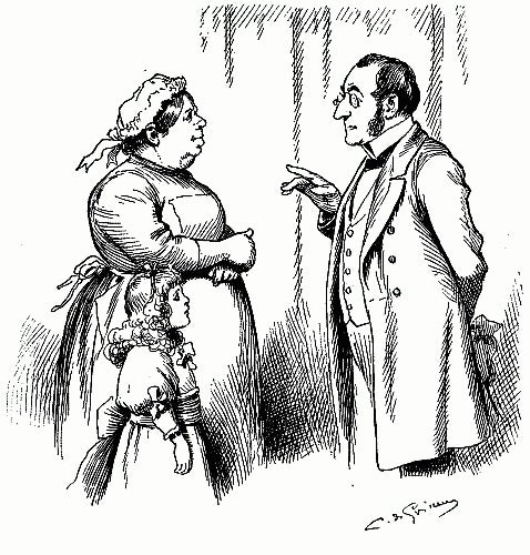
Consider the above line drawing, from an 1893 Funk & Wagnalls publication. Before the computer can begin to identify complex features like eyes, ears, noses, heads, it needs to master very simple features like lines and borders. For example, the line of the man’s chin.

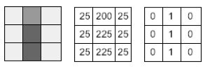
In a typical convolution, the algorithm considers a small area at a time, say three pixels by three pixels. The line at the chin might look like this:

In its first convolution operation, the network could apply a filter operation by multiplying the pixel values by a 3x3 matrix of values that happen to be good at identifying vertical lines, say

The sum of the individual cell multiplications is [0+0+0+200+225+225+0+0+0] = 650. This is a relatively high value, compared to what another arrangement of the filter matrix might produce, because both the image section and the filter have high values in the center column and low values elsewhere. So, for this initial filter action, we can say that the filter has detected a vertical line, and thus we can consolidate the initial nine values of the image section into a single value (say a value between 0 and 1 to indicate the absence or presence of a vertical line).

LOCAL FEATURE MAP

The “vertical line detector” filter moves across and down the original image matrix, recalculating and producing a single output each time. We end up with a smaller matrix; how much smaller depends on whether the filter moves one pixel at a time, two, or more. While the original image values were simply individual pixel values, the new, smaller, matrix is a map of features, answering the question, “Is there a vertical line in this section?”

The fact that the frame for the convolution is relatively small means that the overall operation can identify features that are local in character. We could imagine other local filters to discover horizontal lines, diagonal lines, curves, boundaries, etc. Further layers of different convolutional operations, taking these local feature maps as inputs, can then successively build up higher level features (corners, rectangles, circles, etc.).

A HIERARCHY OF FEATURES

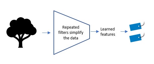
The first feature map is of vertical lines; we could repeat the process to identify horizontal lines and diagonal lines. We could also imagine filters to identify boundaries between light and dark areas. Then, having produced a set of initial low-level feature maps, the process could repeat, except this time working with these feature maps instead of the original pixel values. This iterative process continues, building up multidimensional matrix maps, or tensors, of higher and higher-level features. As the process proceeds, the matrix representation of higher-level features becomes somewhat abstract, so it is not necessarily possible to peer into a deep network and identify, for example, an eye.

In this process, the information is progressively compressed (simplified) as the higher-level features emerge:

THE LEARNING PROCESS

How does the net know which convolutional operations to do? Put simply, it retains the ones that lead to successful classifications. In a basic neural net, the individual weights are what get adjusted in the iterative learning process. In a convolutional network, the net also learns which convolutions to do.

In a supervised learning setting, the network keeps building up features to the highest level, which might be the goal of the learning task. Consider the task of deciding whether an image contains a face. You have a training set of labeled images with faces, and images without faces. The training process yields convolutions that identify hierarchies of features (e.g., edges > circles > eyes) that lead to success in the classification process. Other hierarchies that the net might conceivably encounter (e.g., edges > rectangles > houses) get dropped because they do not contribute to success in the identification of faces. Sometimes it is the case that the output of a single neuron in the network is an effective classifier, an indication that this neuron codes for the feature you are focusing on.

UNSUPERVISED LEARNING

The most magical-seeming accomplishment of deep learning is its ability to identify features and, hence, objects in an unsupervised setting. Famous examples include identifying images with faces and identifying dogs and cats in images. How is this done?

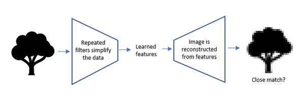
One method is to use a so-called autoencoder network. These networks are trained to reproduce the input that is fed into them, by first creating a lower-dimension representation of the data and then using the created representation to reproduce the original data. The network is thus trained to retain the features that facilitate accurate reproduction of the input.  

Viewed in the context of our image example, autoencoders have the following high-level architecture:

Up to the learned features point (the bottleneck in the image), the network is similar to the supervised network. Once it has developed the learned features, which are a low-dimension representation of the data, it expands those features into an image by a reverse process. The output image is compared to the input image, and if they are not similar, the network keeps working (using the same backpropagation method we discussed earlier). Once the network reliably produces output images that are similar to the inputs, the process stops.

This internal representation at the bottleneck now has useful information about the general domain (here, images) on which the network was trained. It turns out that the learned features (outputs of neurons at the bottleneck) that emerge in this process are often useful. They can be used, for example, for building a supervised predictive model or for unsupervised clustering.  

THE BOTTOM LINE

The key to convolutional networks’ success is their ability to build multidimensional feature maps of great complexity (requiring substantial computing power and capacity) leading to the development of learned features that form a lower-dimension representation of the data. Different convolutional architectures (e.g., types of filtering operations) are suitable for different tasks. The AI community shares pretrained networks that allow analysts to short-circuit the lengthy and complex training process that is required, as well as data sets that allow training and benchmarking to certain tasks (e.g., data sets of generic images in many different classes, images specifically of faces, satellite imagery, text data, voice data, etc.).